


Statistics and Self-Driving Cars
What's the point of high school math? Part 2

Welcome back to the second installment in my back-to-school series! Part 1 contains helpful background information about how computer vision engineers think about cameras, and you can read it here. For Part 2, we’re going to be talking about how statistics can be useful when developing algorithms for self-driving cars.
A key part of developing a self-driving car is localization, or figuring out where you are. GPS is an important component of that, but since it is only accurate to a few feet when in cities, it is not enough. We need to know our location to a few inches in order to avoid pedestrians, stop at red lights, and generally drive in a manner that keeps everyone alive. This is accomplished through a navigation filter and a sensor suite. The sensors in the sensor suite will take measurements as the car drives around, and the navigation filter will extract information from all the measurements and fuse them together to get a more accurate guess of where we are. We can only get a guess because the sensors are noisy - we can have rain obscuring the camera or a GPS interruption or general system malfunction. The idea is that if we get a lot of measurements and update the filter very fast, then we will have a good enough idea of where we are. This is a complicated topic that involves physics and a future article will talk about this in more detail. For now, I want to focus on how we can use cameras to get relevant information for our navigation filter.
Let’s say we know our self-driving car is going to be exclusively driven on the Las Vegas strip, like the Waymo taxis. Las Vegas is a relatively static environment - the Luxor was there yesterday and it’s going to be there tomorrow. Thus, if we know where the Luxor is, and we see the Luxor, then we know where we are. This is similar to the game GeoGeussr, where you are presented with a random Google StreetView photograph and you have to guess where you are. Alternatively, you can think of it as similar someone giving you landmark-based directions - “go left at the red house, if you hit the green mailbox you’ve gone too far”. This type of navigation is called terrain relative navigation (TRN).
Terrain relative navigation comes naturally to humans, but it is trickier to implement in algorithm format. First, we need to prepare a database of reference imagery. These images need to cover the area we plan to drive in, be high-enough resolution to extract information, and be “geo-referenced” (have latitude and longitude coordinates attached to them). The United States Geological Survey as well as private companies such as Maxar and Planet provide this type of imagery. We need it to be geo-referenced so that we have actual numbers to put in our navigation system. There are no humans in the loop while the algorithm is running, so us knowing where the images were taken is not enough. We need it to be high-resolution so that we can get a more accurate guess than what we already have. Remember the GSD (ground square distance) discussed in the previous article - if we know where we are within 10 feet, and the GSD of our reference imagery is 15 feet, then that imagery won’t help us because it can only tell us our location to 15 feet.
Next, we put that database on our self-driving car. As we drive around, we take a picture. We can use our navigation filter to get an estimate of where we are. Based off our estimate of where we are, we can pull out images from our database that we expect to see. It’s unlikely that the picture we take will exactly match the pictures in our reference imagery, so we will pick out smaller patches of the image, called “landmarks” to look at in more detail. There are lots of ways to pick out landmarks, but for now let’s say we just picked a grid. The idea is that even if we don’t have an exact picture map, at least some of these landmarks will appear in our reference images.
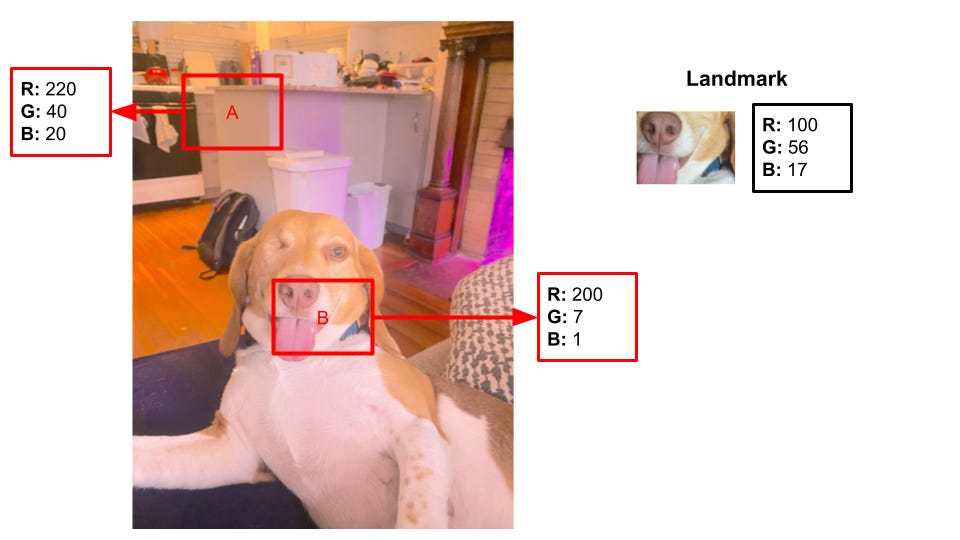
Now, we have our landmarks and our reference images. A human can easily see what part of the images match with the landmarks, but remember that a computer only sees the pixels and doesn’t have a high-level understanding of the image. So, we use math to compare the landmark to the references images. Starting at the top corner of the reference, we add up the absolute differences in pixels between the sub-section of the reference image and the landmark. Then, we move over one pixel and start again. After we’ve gone over the entire reference image, we pick the area that is the closest in terms of pixels to our landmark and say “this area of the reference image is the same area as we see in the landmark”. The picture of Penny below illustrates how this works.

We have a landmark with the pixel values (100, 56, 17). Humans can clearly see that Patch B (110, 58, 17) is a better match than Patch A (200, 7, 118). The computer needs the pixel values to see it - notice how the values of B are much closer to the values of the landmark than Patch A. This is because Patch B imaged the same area as our landmark, so it has stored the same values. The computer will calculate:
Patch A vs. Landmark:
Patch B vs. Landmark:
Comparison:
and determine that Patch B is a better match because it is closer than Patch A in terms of pixels. This works great when the conditions of the database images match the conditions of the image we are taking. Imagine instead that we have our same reference database, but we take a picture with the camera on and it becomes overexposed:
We can clearly see that Patch B is still a better match than Patch A, but can the computer? Let’s do the same math:
Patch A vs. Landmark:
Patch B vs. Landmark:
Comparison:
Now our algorithm thinks that Patch A should be a match! This sensitivity is a big weakness - we don’t want our self-driving car to be limited to just times where we have reference imagery for it. There are a couple ways that we can account for this, and the best solution depends on the end use case of our images.
First, let’s consider a case where all of our images and landmark patches have roughly the same ground square distance. Thus, Penny will take up roughly the same amount of space in one picture as another. We would then expect similar ratios of light and dark in each image, even if the absolute value of the images are different - Penny will still be the same colors, but different cameras and lighting conditions will result in those colors being stored in different ways. We can recover the ratios by normalizing each pixel using the equation:
This normalization, called “linear normalization” in statistics, will allow us to get this apples-to-apples ratio comparison. Pixel values can range from 0 to 255, but often one image does not contain that much variety. Instead, we could have a landmark with green values ranging from 50 to 100 and a corresponding patch with values ranging from 75 to 120 in an image with different lighting. This normalization will transform those values so that they are now scaled between 0 and 1, and thus we can compare them directly.
Next, let’s consider a case where we might not expect the ground square distance of the database images to match the images we are getting. Pretend we are getting closer to Penny and now our images start to look like this:

A human can easily deduce that this is a close-up of Penny’s leg. However, the ratio of colors in this image do not match the image above that forms our database - there is much more red, and almost no blue or green. Thus, if we were to do linear normalization on this, we would not be doing a direct comparison. However, we still have pictures of Penny in our database, and we do know what sort of ratios we should be seeing in a picture of her leg. So, instead of normalizing by the values in the image alone, we can normalize by the values of our entire data set:
This form of normalization, called z-score normalization, will scale the pixels in the image so that have a mean of 0 and a standard deviation of 1 relative to the entire dataset. This normalization is better for cases where we expect similar distributions of colors in our reference database and our real-time images, such as when the database camera and in-car camera are the same. Sometimes, it makes sense to perform both normalizations.
Now, we will repeat this for all the landmarks we have and get a collection of landmarks that are matched to areas in our geo-referenced database images. This is where the algebra starts to come in…