


Physics and Self-Driving Cars
What's the point of high school math? Part 6

This is the sixth installment in the “What’s the point of high school math?” series, where I walk through the process of programming a self-driving car to “see” and navigate its environment and discuss how high school math is relevant. Part 1 introduces the terminology that computer vision engineers use to talk about such a problem. Part 2 covers statistics, Part 3 talks about algebra, Part 4 brought us to geometry, and Part 5 covered miscellaneous AP classes. Now, we have created a terrain relative navigation system that can take a live photo of our environment and a guess of where we are and give us a more accurate estimate of our location. This is useful, but if we want our car to be able to react in real-time to decisions, we also need to predict where we are going next.
One way that we could do this doesn’t require any of our TRN solution - we can just use a $5 accelerometer to get the acceleration of our vehicle, and use the classic physics equations:
In theory, this should be all that we need. Unfortunately, in practice no sensors are perfect, and small amounts of noise are introduced with every measurement we take. These errors can be minuscule, but because each prediction depends on all the previous predictions, the errors will add up over time and cause our estimates to diverge.
This is where the concept of a navigation filter comes in. Navigation filters such as Kalman filters and particle filters recognize that while accelerometers are cheap, they are prone to error, and other sensors can help with that. Most navigation filters consist of two steps - an estimation step, and an update step. The estimation step is just what it sounds like - we can use equations like the physics equation above to guess where we will be at any given time. The update step is also self-explanatory - we get actual measurements from our sensors, plug them into the relevant equations, and fuse them together to get our guess.
For example, let’s imagine we have a very simple system of our accelerometer and TRN system. For every photo we take, we will also take a measurement from our accelerometer. We will then have two measurements - our acceleration, from the accelerometer, and our pose estimate, from our TRN system. We will then feed those measurements to our navigation filter. This filter will first try to guess what the final output position will be based off its state space model. The state space model is just a combination of equations, like the physics one shown above, that match with whatever sensors we are using. This is the estimation step.
Next, for the update step, the filter will use the same fusing math as the prediction step, but using the actual measurements we have. By comparing the difference between the actual value and the predicted value, the filter will decide what variables to update in the state space model to better represent what is actually happening. The filter can then tell us our position right now, and also at any time in the future, based off what equations are used.
This is all well and good, but I skipped over a vital part of this algorithm - how do we decide how to fuse the measurements from different sensors? One easy way is to simply take an average of all the positions our different measurement models calculated. However, let’s say we recieve a picture like this:
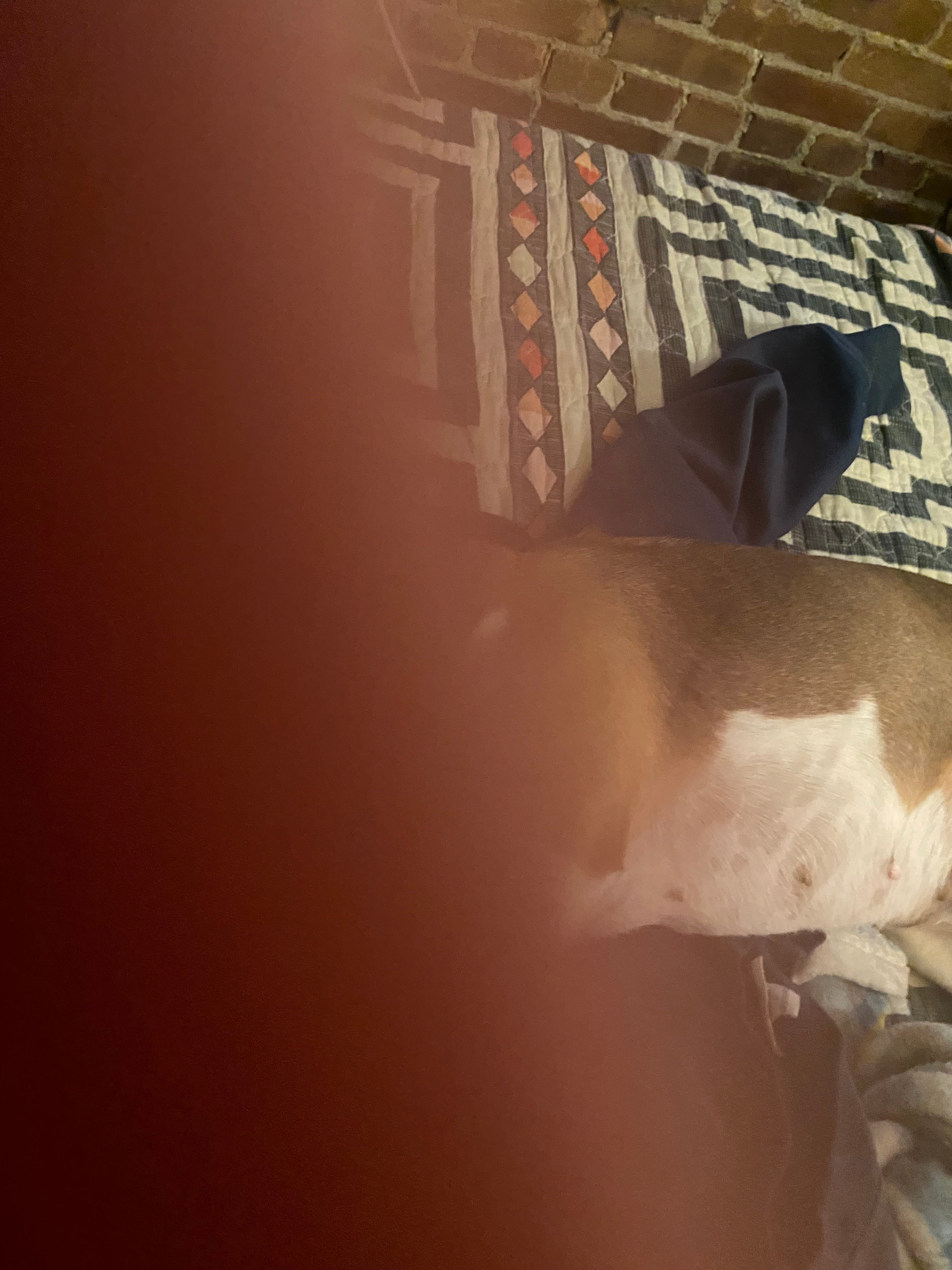
Humans can clearly see that Penny is lounging behind my finger, but remember the weakeness of TRN we talked about in previous articles - this is going to cause us to have bad landmark matches with our database, and thus our guess of position is going to be very off. We wouldn’t want to weight this measurement the same as our normal accelerometer measurement, or as much as other TRN measurements, since we know it’s not very good.
Navigation filters get around this issue in two ways. If you know for certain that one of your sensors is better than the other, you can do a weighted average and have every TRN measurement count for 2x the weight of an accelerometer measurement. On a per-measurement basis, we account for this uncertainty by calculating the covariance of each sensor measurement along with its position. This covariance is traditionally calculated based off information about the given sensor and what you know about your enviornment, but newer methods are looking into performing machine learning on the individual measurement. Covariance tells us how confidence we are in that specific measurement, and it is updated along with position in our filter. Covariance is also used while deciding how to fuse the measurements.
Once our navigation filter is properly tuned to our sensors, we can guess where our car is to within a few feet, as well as how confident we are in that prediction. This prediction is then used by other algorithms to decide where the car should go next. Of course, this all assumes the car can drive anywhere it wants, and anyone who has ever been outside knows that is not true…